1
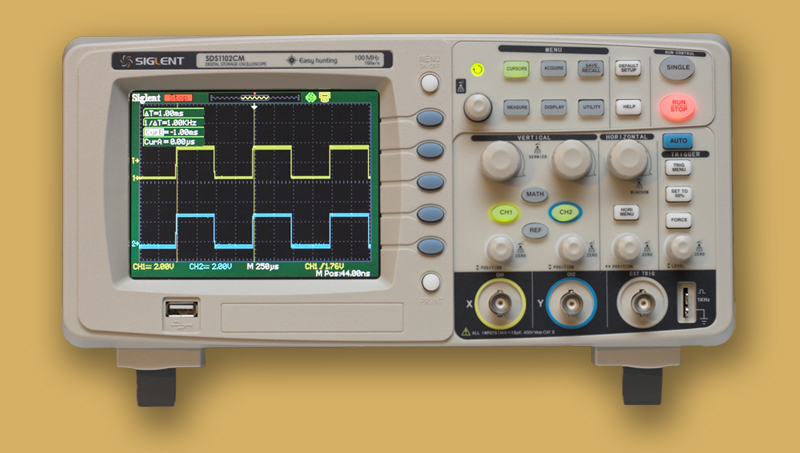
SIGLENT SDS1102CM 2x100MHz, 2x500Msa/s, 2x1Msa memory depth
oscilloscope review
Where I found some faulty operation,
or function that is useable only with special oscilloscope settings I colored
the text to dark red. If you are interested in the usability
of any additional feature or you found any of my tests faulty, or you have a
better idea for using any function please mail me. I will try it if I have
the possibility and add it to the review.
1.1 Instruments used
SIGLENT SDS1102CM Based on the CSV file: Model Number: SDS1102CM Serial Number: SDS00002111512 Software Version: 3.01.01.22 Based on the turn on screen: Software Version: 3.01.01.223 Approx. 450USD on ebay.com Agilent Technologies DSO6054A 500MHz 4Gsa/s 4Msample/ch memory depth 7000USD on ebay.com Agilent Technologies DSO-X 3024A 1channle: 4Gsa/s (Interleaved) 2-4channel: 2Gsa/s 200MHz bandwidth Approx. 3500USD at hu.rs-online.com 1.2 Bandwidth limit
I tested the bandwidth limit by an
1Vpp sine wave at 100MHz. The reference instrument was a Tektronix 500MHz
oscilloscope. The display at 10MHz was identical on the two scopes. At 100MHz
I measured about 0.7Vpp on the SDS1102CM, while the Tektronix still measured
1Vpp. The bandwidth limit of the SDS1102CM is really 100MHz 1.3 Memory depth
The memory depth is 1Mpoints/channel,
as it can be seen from the CSV file header. See the spectrum measurements.
The point in this test is to analyze that if I stop the acquisition than how
detailed information can be seen in the signal by zooming into it. |
 E-MAIL
|
This is an SPI communication at 8MHz clock.
In a 25us/div setting one packet of data does not fill the screen. The packet
time (16 byte) is about 32us, so the screen is now about 150 bytes long.
(Plus the dead time.) Settings -
Memory Depth: LongMem -
Trigger: |
|
|
Zooming on one byte of data, the data
can be read from the screen, but it is at the very limit. (Data clocked by
rising edge, 00010100) The zoom ratio is 25us/100ns = 250 |
|
|
Here is the same view extracted from
the 2x1Mpoint CSV file by Matlab. So what can be seen on the picture that is
really the whole information in the memory. |
|
|
The signal in Matlab seems to be more
smooth, some extra oscillations are missing from it. This is caused by the “sinx/x:
sinx” setting. If I set it to “x” the oscillations disappear and we can see
the pure data. This seems to be identical to the Matlab curve. |
|
|
Now the same packet fills the screen. |
|
|
Examining only one byte is quite easy
by zooming on it. The zoom ratio is 5us/100ns = 50 The signal is stopped by pressing the
SDS1102CMs STOP button in It must be also noted that the 2Mpoints
memory depth works only at 50ms/div and faster time/div settings. |
|
|
I got the information that in earlier
firmwares (1.01.01.07R13) the signal saved in SINGLE mode is less detailed than
if the signal is stopped by the STOP button. I tested the memory depth again by
stoping the signal with the SINGLE button, or switching the trigger mode to
SINGLE. Both cases I got the same detailed picture as in the above case. This
is the header of the CSV file saved in SINGLE mode. The record length is
1048576 points per channel. |
Record Length,1048576,,Source,CH1,CH2 Sample Interval,CH1:0.0000000100000
CH2:0.0000000100000,,Second,Volt,Volt Vertical Units,CH1:V
CH2:V,,-0.00524288000,0.00,4.32000 Vertical Scale,CH1:2.00
CH2:2.00,,-0.00524286969,-0.08000,4.32000 Vertical Offset,CH1:2.00000
CH2:-6.16000,,-0.00524286000,0.00,4.24000 Horizontal Units,s,,-0.00524284969,0.08000,4.24000 Horizontal
Scale,0.0000050000,,-0.00524284000,0.00,4.32000 Model Number,SDS1102CM,,-0.00524282969,-0.08000,4.32000 Serial
Number,SDS00002111512,,-0.00524282000,0.00,4.24000 Software
Version,3.01.01.22,,-0.00524280969,0.00,4.24000 ,,,-0.00524280000,0.00,4.24000 ,,,-0.00524278969,0.00,4.32000 ,,,-0.00524278000,-0.08000,4.32000 ,,,-0.00524276969,0.00,4.16000 ,,,-0.00524275969,0.00,4.16000 |


1.4 Sampling rate and “dots” display
|
Settings -
Memory Depth: LongMem -
2 channel -
2.5ns/div -
Stopped by SINGLE button -
Display/Type: dots The sampling rate displayed by the
SaRate field in Acquire menu is 250Msa/s. I expected 500Msa/s in the fastest
time/div setting with two channels active. The cursor reads between two displayed
samples 500MHz. Maybe, the SaRate field is wrong… If I stop it by the STOP button I get a
faulty display, see later… |
|
|
I’d like to see 1Gsa/s, so I turned
off CH2. Now the SaRate field in Acquire menu is 500Msa/s. Here it is stopped by the SINGLE
button, so the correct data can be seen. The distance of the dots is also
correct. |
|
|
Here it is stopped by the STOP button,
so the displayed data is faulty like with the previous settings. |
|
|
I turned off the LongMem. Settings -
Memory Depth: -
1 channel -
2.5ns/div -
Stopped by SINGLE button -
Display/Type: vectors |
|
|
If I turn the vectors off I can
finally see 1Gsa/s in the SaRate field and on the screen also. The STOP/SINGLE problem is also
solved, I see the same if I stop it either way. |
|


1.5 Equivalent time sampling
|
This is the falling edge of the
previous SPI clock and the rising edge of the data. On the running picture there is not
big difference between the two interpolation settings. (Sinx/x = x or sinx) Also there is no difference between
Display Type = Vectors or Dots, although there should be difference, because
in this case one sample is taken only in every 2ns. If the sampling is stopped the dots can be seen. Settings -
Memory Depth: LongMem -
Trigger: -
Mode: Real Time |
|
|
If I switch to Mode: Equ Time I have to wait 10 seconds to get this display. It seems as if the signal was recorded
in a much slower time/div setting. This must be some
software fault. |
|


1.6 Undersampling
|
I use a 15.041kHz sine wave. Settings -
Acquire: Sampling -
Trigger: |
|
|
The signal is stopped at 500ms/div. In
this setting no undersampling can be seen. The signal is a yellow strip. If I zoom into it to 5ms/div I can see
it to be a 45.05Hz sine wave. This effect is a consequence of the sampling
theorem, but care must be taken. |
|
|
Let’s justify this with the Agilent.
The Agilent has an “antialiasing” function that can be switched off. Its own
calibrating signal (1.2kHz) can not be undersampled in any time/div setting. This is a 27MHz clock signal. |
|
|
With the antialiasing turned off, and
the signal stopped at 200ms/div, zooming into it the undersampling can be
seen. If the antialiasing is ON, than we get
some sawtooth signal at the same amplitude, that I don’t understand, but at
least it can not be mixed up with a 95.7Hz clock… |
|


1.7 Trigger
|
The signal is the calibrating signal
of the SDS1102CM. 3Vpp, 1kHz Settings -
Trigger: -
Trigger level: 1.12V -
Trigger edge: falling -
Stopped by STOP button I should be able to see a falling edge
at the trigger point. |
|
|
If I set the trigger level slightly
higher the display gets better, but far from perfect. Settings -
Trigger level: 1.68V |
|
|
The level is not changed, just the
time/div setting. The signal is still stopped by the STOP button. The trigger
edge is still falling! In this case the running signal is
jumping in time, as if there was no trigger at all. |
|
|
Same settings, but the signal is
stopped by SINGLE button. Seems to be good. While running it is still similar to the previous picture. |
|


1.7.1 Trigger point
|
Although in the “Equivalent time sampling”
chapter it was clear that the falling edge of the signal crosses the trigger
level at the trigger time point, there are problems with the trigger time
point in many settings. Settings -
Trigger: The SPI data packet is stopped here
with the STOP button. While the signal is running the trigger
is at the first rising edge of the yellow channel, but if it is stopped it
waits about half second, and makes last sweep. But the trigger time is not
correct. |
|
|
If I stop the same signal by SINGLE
mode than the trigger point is in the right time. In different settings it happens that
the SDS1102CM forgets to display the signal at the trigger point. |
|


1.7.2 Pre triggering
|
The trigger point is pushed to the left
by 31.54us. In this time/div setting (250ns/div) the trigger point is on the
very left side of the record as it is shown by the red ’T’ at the top of the
screen. The trigger point can not go out of the record, so further decreasing
the time/div is not possible. |
|
|
If I still try it I get some false
result. Neither the signal display is correct, nor the
trigger point mark at the top of the screen. |
|


1.8 Dual time base, Delayed signal
|
Instead of the pre trigger the dual time
base can be used. I still use the SPI communication. 16bytes in every 10ms,
as it can be seen on the top of the screen. Settings -
Memory Depth: On the bottom it does not turn out
that one packet is 16 bytes. The signal at the bottom is about
50us long, although the data packet lasts only to 32us. On the bottom some trigger problem can
be seen. The green trigger point is far from the beginning of
the signal. |
|
|
Settings -
Memory Depth: LongMem This, or something similar useless and
very faulty display can be seen at changing to LongMem, every time changing
the delayed signals time/div setting, after pressing STOP, and most of the
times pressing the SAVE button. |
|
|
After pressing STOP twice (stopping and
restarting the display) this is the running display. If I press SAVE, mostly I get the previous type of picture, but
sometimes a good one can be caught. The running picture seems to be
perfect. The length of the data packet is correct |
|
|
How about resolution? I still can only
catch the signal by pressing SAVE until I get a good display. The resolution is much better than in
pre-trigger mode, or by zooming on the stopped signal. The time/div ratio is
5ms/25ns=200000 |
|


1.9 FFT, spectrum measurement
1.9.1 How can I get the instrument to
show a very simple spectrum
|
A 15kHz sine wave. Settings -
Memory Depth: LongMem |
|
|
I just turn on the FFT. Settings -
Zoom: 1x -
Cursors: 10MHz, 20MHz From the cursor readouts it can be
seen, that this FFT is useless. Frequencies in the 10MHz range can be read
from it, but the 15kHz can not be seen. |
|
|
I change the sec/div setting to
50ms/div. It can be seen in the Undersampling chapter, that this oscilloscope
can undersample the signal. (For any setting change in the time domain signal
I have to turn the Math channel off, otherwise the buttons set the FFT.) There is nothing around 15kHz as the
cursor shows. |
|
|
Go back to a non-undersampling
time/div setting, although in this setting the signal can not be seen, only a
yellow strip. Settings -
Time/div: 1ms/div -
FFT zoom: 10x There is a big peak on the spectrum,
but it is at 600kHz, and the 15kHz peak still can not be seen. |
|
|
Settings -
Memory Depth: Now the 15kHz component can be clearly
seen. It must be noted, that the spectrum is
the same as in the „LongMem” case. I have no explanation for this, but it is
misleading. |
|


1.9.2 Comparison of the spectrums and
the CSV file
|
This is a 1kHz, 3Vpp squarewave, the
calibration signal of the SDS1102CM. The target is to compare the spectrum
calculated by SDS1102CM and by Matlab on a PC using the CSV export of the
scope. |
|
|
I measure the spectrum of this signal
based on the experiences of the previous chapter. Settings -
Window: Rectangle (Because I
will use the same in Matlab) The data of the first peaks is the
following: 1.01kHz: 4.8dBV 3.01kHz: -3.2dBV (difference: 8dB) I suppose these values are correct.
The difference should be 9.62dB, but the error of the reading is big, and the
squarewave can be imperfect. |
|
|
Settings for CSV save: -
This is the header of the CSV file.
The Normal Memory Depth results 20480 points. Other info: 20us/sample,
25msec/div, 1V/div, etc…The first column is the time, not the spectrum! I examined a Long Mem CSV header, the
Record Length was 2097152 points for one channel and 1048568 for two
channels. The file size was about 57MB, the saving to the USB pen lasts about
5 minutes. |
Record Length,20480,,Source,CH2 Sample Interval, CH2:0.0000200000016,,Second,Volt Vertical Units, CH2:V,,-0.20480001563,0.04000 Vertical Scale, CH2:1.00,,-0.20478001563,0.04000 Vertical Offset, CH2:0.00,,-0.20476001563,0.04000 Horizontal Units,s,,-0.20474001563,0.04000 Horizontal
Scale,0.0250000000,,-0.20472000000,0.08000 Model Number,SDS1102CM,,-0.20470001563,0.00 Serial Number,SDS00002111512,,-0.20468001563,0.08000 Software Version,3.01.01.22,,-0.20466001563,0.04000 ,,,-0.20464001563,0.04000 ,,,-0.20462000000,3.12000 ,,,-0.20460000000,3.12000 ,,,-0.20458001563,3.12000 ,,,-0.20456001563,3.12000 ,,,-0.20454001563,3.12000 ,,,-0.20452001563,3.12000 ,,,-0.20450000000,3.12000 ,,,-0.20448000000,3.12000 ,,,-0.20446001563,3.08000 |
|
Out of the data of the CSV file the
Matlab calculates this spectrum. The sampling frequency is 50kHz, the number
of points is 20480, so in the spectrum one point (horizontal axe) is
2.4414Hz. The data of the first two peaks: 1003.41Hz: 15207 3002.92Hz: 6287 The difference is: 7.67dB The 8dB difference measured by the
SDS1102CM is exact. |
|


1.9.3 Spectrum measurement on
complicated signal
|
The signal is the voltage on a small
electric motor in AC coupling. A 22ohm resistor was serial connected with the
motor to make the voltage ripple more visible. The base frequency seems to be
51.02Hz. (See cursors) So I expect a base harmonics at about
50Hz, and one harmonics at every odd multiple of it (150, 250…). And I expect
a higher harmonics at every even multiple also, because visually the signals
frequency seems to be 100Hz. |
|
|
In the FFT nothing can be seen. Settings -
Window: Rectangle (Because I
will use the same in Matlab) I could not find a time/div setting
where the spectrum is visible although if I stop the signal at 1s/div and
zoom into it the waveform can be seen. So I suppose the SDS1102CM
does not use the whole data in the memory to calculate the spectrum. |
|
|
I will calculate the spectrum with
Matlab. This is the first 1000 point in a CSV file saved with 100ms/div
setting. In this case the largest possible resolution of the FFT on the
SDS1102CM is 625Hz/div. So the 50Hz base frequency can not be seen. The base period is about 510points,
the sampling period was 40us. So the period is 20.4ms, and the frequency
49.01Hz. |
|
|
This is the whole FFT of the CSV data.
One point is Fs/20480=1.2207Hz |
|
|
This is the first 300 points of the
FFT. The peaks are at (from the detailed
Matlab analysis): 50.04Hz 98.87Hz 148.92Hz So saving the signal in CSV and
analyzing by Matlab gives a very useable result. The FFT of the SDS1102 is not useable for this. |
|


1.9.4 The same signal on a “more”
expensive scope
|
I tried the same measurement on the
Agilent oscilloscope. The base harmonics is 65.6Hz |
|
|
There is a possibility to zoom on the
interesting part of the spectrum, but the base harmonics can not be seen. X1
cursor is at 64Hz. Settings -
Window: Rectangle (Because the
same was used on the SDS1102CM) The reason can be the rectangular
window function. Only some periods are in the window, and the window width is
not a multiple of the period. |
|
|
If many periods are in the window the
spectrum can be seen as it is expected. I suppose the selected part of the
spectrum, about 500 point is calculated from the 4Mpoints stored in the
memory. |
|


1.10Save
1.10.1 Waveform save
Recalling a saved waveform -
It loads the saved screen with
the settings and stops the display -
Zoom and delay can be adjusted, approximately
according to the Normal MemDepth even if the waveform was saved in LongMem
setting -
If I press the STOP button to
start the scope, the saved waveform disappears. It can not be compared to the
running signal, but it can be saved to picture or CSV -
When saving while the signal is
running it happened (sometimes) that the saved signal jumps somewhere else. -
At recall sometimes nothing is
loaded 1.11REF
The below case was the only one when I
could display the reference signals. At any other try I pressed the SAVE
button on the REF menu it says “Store Data Success”, displays the “A->”
symbol that marks the zero level of the REF signal, displays that the REF is
ON in the menu and DOES NOT display the signal. |
|
Switching between REFA and REFB must be
done on the running signal. If it is done on the stopped
signal, the signal jumps in time, so something else will be saved. The displayed reference signals can be
saved to picture or CSV. The reference signals do not zoom by
setting the time/div. |
|

1.12Noise, Offset
|
The most sensitive settings: 1x probe: 2mV/div, 10x probe: 20mV/div In the tests I always adjusted the
probe setting in the CH1 menu according to the physical probe setting. With both
1x and 10x probe setting at the most sensitive V/div the bandwidth limit is
automatically turned on, and can not be turned off. In the second most
sensitive setting (5/50mV/div) it can be set to be off. Right after turning on the
oscilloscope with both 1x and 10x probe setting the offset of the scope is 1
div (2/20mV) even in AC coupling. The noise is about 0.5 div peak to peak. The following tests were done after 20
minutes warming up. |
|
I connected a 28.8ohm(DC) resistance
earphone speaker to the probe, and whistled in it. Settings -
1x probe -
2mV/div -
AC coupling |
|
|
Keeping the above settings I shorted
the input of the probe. A slight offset can be seen, and a
small noise. The same can be seen in DC coupling. |
|
|
Same settings as above, but with 10x
probe. The result is the same. |
|
|
The same settings again, but after an
automatic calibration. The noise is much smaller and the
offset can not be seen. So if noise is critical it is worth to
make a calibration. |
|


1.13Signals around the badwidth limit
of the scope
|
An application
note of Agilent states that sampling fidelity can often be more important
than maximum sample rate. For evaluating sampling fidelity I used one single
output of a 155.52MHz VCXO. This VCXO is supposed to output a square wave,
the amplitude is about 200mV. I connected an LC network to it to amlify the
fundamental frequency to receive a sinewave. The output of the LC network wa
finally not useable, but it was good for comparing the SIGLENT SDS1102CM to
the Agilent DSO-X 3024A. |
1.13.1 Measurements with Agilent DSO-X
3024A
|
Theoutput of the VCXO. The bandwith of
this scope is 200MHz, so the amplitude of the fundamental harmonics must be
real here. About 400mVpp. Settings -
AC coupling -
Window: Hanning -
10ns/div -
Sampling: 4Gsa/s, since only one
channel is on, the sampling is interleaved. -
FFT: 0 – 1GHz, 100MHz/div No problem can be seen on the signal,
no distortion. It seems to be sine, although the spectrum shows some
harmonics. The haronics are the multiples of
157MHz: 157, 310, 466, 646, 955 The application note says that the
error of the interleaved sampling causes harmonics at Fsampling-Fsignal.
Where Fsampling is the sampling frequency of one AD converter of
the two. That would be here about 1.85GHz. This can not be seen on this
picture. If I turn on the bandwith limit for channel
1 the signal totally disappears, as it is expected |
|
|
This is the output of the LC filter in
10ns/div again. It is quite noisy, the spectrum does not show any 155MHz
harmonics. A 100MHz peak can be seen on the
spectrum, and some slight feeling of a 100MHz sine on the time domain signal.
|
|
|
Here the same signal is averaged out
of 256 shots. The amplitude can not be measured, but
the spectrum is interesting. It is clear that there is the fundamental
frequency of the VCXO. Additional frequencies are at the
multiples of 100±10MHz. I suppose this is the error of the signal source. |
|


1.13.2 The same signals measured by the
SDS1102CM
|
This is the output of the VCXO. The
signal is jumping, two shots are always different, many shots can be seen on the screen in the same time. The memory depth is Settings -
AC coupling -
Sampling: 1Gsa/s, since only one
channel is on, the sampling is interleaved. -
Sinx/x: x |
|
|
Here is the above signal stopped. On the Agilent this was a sinewave
with a constant amplitude, but this signal is over the specification of this
scope. |
|
|
When turning on the averaging a
constant sinewave and the jumping shots can be seen in the same time. If I stop the signal the averaged constant sine disappears and I get
the same as in the above picture. Settings -
Averaging: 128 |
|
|
The output of the LC filter. Unlike
the Agilent the SDS1102CM shows a significant amplitude. Is it +1 point for
the Siglent! The amplitude is approximately 60mVpp. |
|
|
If I turn the bandwidth limit on, the amplitude
is still about 30mVpp, although the signal should disappear. It can be stated, that the 100MHz
could be seen on the Agilent scope also. |
|
|
The output of the VCXO again. It seems
like amplitude modulated. I suppose this is the result of the SDS1102CM
sampling system. |
|
|
I turned the Sinx/x interpolation on,
to see how distorted is the signal when using the 1GHz interleaved sampling
of the scope… |
|
|
… and I compared to the 500MHz non
interleaved sampling. (CH2 is on) I can see no difference. According to
the application note this shows no error in the sampling system. Or at least
it can not be seen |
|
|
This is the spectrum of the VCXO
output. It is very similar to the LC filter output on the Agilent… I have no
idea why. Spectral components can be seen at
156MHz and its multiples (312, 468). Also there are lines at 100MHz and its
multiples, which also appeared on the Agilent scope. But here a 344MHz component can also be
seen which is the difference of the sampling frequency of one AD and the
fundamental frequency of the signal. This shows some alignment error in the
interleaved sampling. |
|
|
The spectrum of the output of the LC
filter does not contain the 156MHz. (Like on the Agilent without averaging)
but it contains the 100MHz and its multiples. On the SDS1102CM I can not use the
averaging function for getting a more clean picture, because it does not work
for the FFT As it is measured on both scopes this
can be the error of the signal source. |
|


1.13.3 A 66MHz clock, that the SDS1102CM
can deal with
|
The signal seems to be a sinewave,
although it is a squarewave. This is normal, the harmonics are filtered. The multiples of 66MHz can be seen. I can’t explain the multiples of 33Mhz
that can also be seen. The amplitude of the harmonics is
decreasing, except around 433MHz. I suppose this part
is caused by the misalignment of the interleaved sampling. |
|

1.14Display problems
|
While the signal is running and the
scope is set to dot display mode the dots are very dense on the screen. As if it was some equivalent sampling mode. |
|
|
When I stop the signal it shows the
normal density of dots. |
|


|
The averaging function works only while
the signal is running, and it works only in AUTO trigger mode. See the figures in the “The same signals measured by the SDS1102CM”
chapter. |
1.15Edit history
|
03.01.2012. |
First version |
|
05.01.2012. |
“Noise, Offset” added |
|
10.01.2012. |
“Sampling rate and “dots” display”
and “saved signal detail in single
mode test” added |
|
13.01.2012. |
“Signals around the bandwidth limit of
the scope” added “Display problems” added |
|
|
|
|
|
|
|
|
|
|
|
|